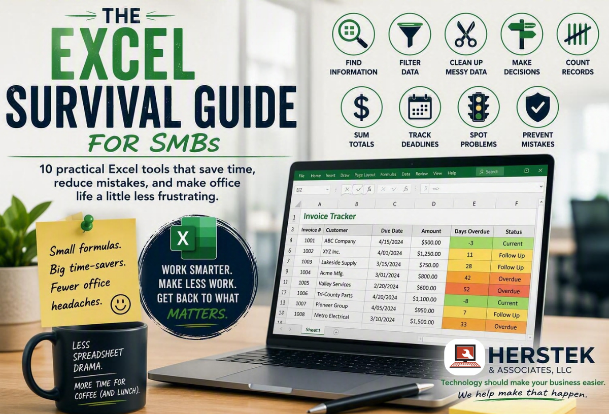
10 practical Excel tools that save time, reduce mistakes, and make office life a little less frustrating.

Estimated reading time: 10–12 minutes
Or about three minutes if you skip directly to the spreadsheet problem currently making you mutter.

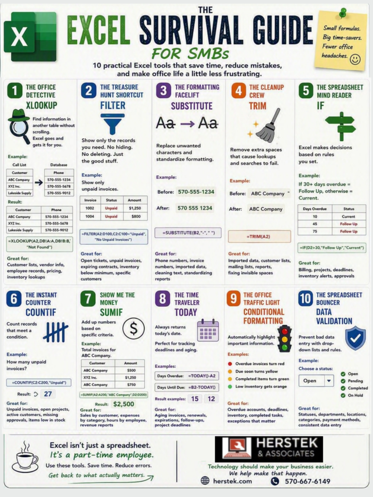
✅ Looking up information? → XLOOKUP

✅ Need a list of unpaid invoices? → FILTER

✅ Cleaning messy imports? → SUBSTITUTE

✅ Fixing hidden spaces? → TRIM

✅ Automating decisions? → IF

✅ Counting records? → COUNTIF

✅ Summing totals? → SUMIF

✅ Tracking deadlines? → TODAY

✅ Highlighting problems? → Conditional Formatting

✅ Preventing bad data? → Data Validation

---

Let’s be honest: most small businesses do not struggle because they lack technology.

They struggle because someone is spending 20 minutes doing something Excel could do in 20 seconds.

Employees search customer databases manually, copy information between spreadsheets, count unpaid invoices row by row, and highlight overdue accounts one cell at a time.

Meanwhile, nearly every office has at least one workbook named something like:

Customer_List_FINAL_Updated_USE_THIS_ONE_v7.xlsx

Excel cannot solve every business problem. But it can eliminate a surprising amount of repetitive work once someone shows you what to ask it to do.

This guide walks through 10 practical Excel tools using ordinary office problems—not intimidating spreadsheet jargon. You do not need to become an Excel expert. You only need to recognize which tool could make the job in front of you easier.

---

What’s Inside This Survival Guide

Need Help Fast?

Skip directly to the solution you’re trying to solve:

Category	Survival Guide Name	Excel Tool	What It Helps You Do
🔍 Find Information	The Office Detective	XLOOKUP	Match information from another customer, vendor, employee, or product list.
🔍 Find Information	The Treasure Hunt Shortcut	FILTER	Display only the records you currently need.
🧹 Clean Up Data	The Formatting Facelift	SUBSTITUTE	Replace unwanted characters and standardize formatting.
🧹 Clean Up Data	The Cleanup Crew	TRIM	Remove extra spaces that interfere with searches and formulas.
🤔 Make Decisions	The Spreadsheet Mind Reader	IF	Display different results based on rules you define.
🔢 Answer Questions	The Instant Counter	COUNTIF	Count records that meet a particular condition.
💰 Calculate Totals	Show Me the Money	SUMIF	Total sales, expenses, hours, or balances by category.
📅 Track Deadlines	The Time Traveler	TODAY	Calculate overdue days, upcoming deadlines, and expiration dates.
🚦 Spot Problems	The Office Traffic Light	Conditional Formatting	Automatically highlight important information.
🛡️ Prevent Mistakes	The Spreadsheet Bouncer	Data Validation	Create drop-down lists and restrict inconsistent data entry.

You don’t need to become an Excel expert to save time.

Most spreadsheet frustrations come from a handful of repetitive tasks that Excel can already handle. The goal is not to turn everyone in the office into a spreadsheet wizard. The goal is to spend less time fighting spreadsheets and more time getting actual work done.

---

Let’s start with the tool that probably saves more office time than any other function in this guide.

1. The Office Detective 🔍

XLOOKUP

Let’s begin with a problem that appears in offices everywhere.

You have an Excel file open containing a list of companies that need to be called.

Customer Call List

Customer	Phone
ABC Company
XYZ Inc.
Lakeside Supply
Acme Manufacturing

The customer names are there, but the phone numbers are missing.

The phone numbers do exist. Unfortunately, they are buried inside another Excel file containing hundreds—or thousands—of customer records.

That larger database may include columns for:

• Customer name
• Phone number
• Email address
• Mailing address
• Primary contact
• Account balance
• Account manager
• Renewal date

You only need the phone numbers.

Without XLOOKUP, you would have to:

1. Open the customer database.
2. Search for the first company.
3. Locate the correct phone number.
4. Copy it.
5. Return to the call list.
6. Paste it.
7. Repeat the process for every company.

That may be manageable for four customers. It is a very different afternoon when the list contains 400.

XLOOKUP searches a specified range for a value and returns corresponding information from another range. In this example, Excel uses the company name to locate and return the matching phone number.

A Real-World XLOOKUP Walkthrough

For this example, imagine that you have two Excel files:

File 1: Customer Call List.xlsx

Column A	Column B
Customer	Phone
ABC Company
XYZ Inc.
Lakeside Supply
Acme Manufacturing

File 2: Customer Database.xlsx

Column A	Column B	Column C	Column D
Customer	Phone	Email	Contact
ABC Company	570-555-1234	info@abc.example	Jane
XYZ Inc.	570-555-5678	info@xyz.example	Mike
Lakeside Supply	570-555-9012	info@lakeside.example	Sarah
Acme Manufacturing	570-555-4567	info@acme.example	Tom

Our job is to match each company in the call list with the correct phone number in the database.

Step 1: Open Both Excel Files

Open:

• Customer Call List.xlsx
• Customer Database.xlsx

Keeping both files open makes building the formula easier because you can select the correct ranges instead of typing the workbook references manually.

Step 2: Select the First Empty Phone Cell

Return to the Customer Call List and click cell B2, the empty cell beside ABC Company.

This is where the first phone number should appear.

Step 3: Begin the Formula

Type:

=XLOOKUP

Excel is now waiting for directions.

Step 4: Select the Company You Want to Find

Click cell A2, which contains ABC Company, and type a comma.

The beginning of the formula will look like this:

=XLOOKUP(A2,

“Excel, take the company name in A2.”

That company name is the clue Excel will use to search the database.

Step 5: Select the Company Names in the Database

Switch to Customer Database.xlsx.

Select the company-name cells in Column A.

For example:

A2:A1000

Then type another comma.

Excel will insert the workbook and worksheet information automatically. The formula may now resemble this:

=XLOOKUP(A2,‘[Customer Database.xlsx]Customers‘!$A$2:$A$1000,

Do not let the brackets, dollar signs, or workbook name scare you. Excel adds those details because the information is stored in another file.

Office translation

“Look for that company name in the customer-name column of the database.”

Step 6: Select the Phone Numbers to Return

Still in the customer database, select the matching phone-number cells in Column B:

B2:B1000

Then type another comma.

The formula may now resemble this:

=XLOOKUP(A2,‘[Customer Database.xlsx]Customers‘!$A$2:$A$1000,‘[Customer Database.xlsx]Customers‘!$B$2:$B$1000,

Office translation

“When you find the company, bring back the phone number from the same row.”

Microsoft calls the first selected range the lookup array and the second selected range the return array. The ranges need to cover the corresponding rows so Excel returns the information associated with the match.

Step 7: Add a Friendly Message for Missing Records

Type:

“Not Found”)

The complete formula will resemble:

=XLOOKUP(A2,‘[Customer Database.xlsx]Customers‘!$A$2:$A$1000,‘[Customer Database.xlsx]Customers‘!$B$2:$B$1000,“Not Found”)

Your workbook and worksheet names will naturally be different.

Office translation

“If you cannot find the company, show ‘Not Found’ instead of an error.”

A missing result could indicate:

• A spelling difference
• An outdated company name
• An extra space
• A customer missing from the database
• The wrong range selected in the formula

“Not Found” gives the employee something understandable to investigate.

Step 8: Press Enter

Excel searches the database for ABC Company and returns:

570-555-1234

Your call list now looks like this:

Customer	Phone
ABC Company	570-555-1234
XYZ Inc.
Lakeside Supply
Acme Manufacturing

Step 9: Copy the Formula Down

Select the formula cell and locate the small square in its lower-right corner.

Either:

• Drag the square down through the remaining rows, or
• Double-click the square to fill adjacent rows automatically.

Excel adjusts the customer reference for each row while continuing to search the database.

Completed Call List

Customer	Phone
ABC Company	570-555-1234
XYZ Inc.	570-555-5678
Lakeside Supply	570-555-9012
Acme Manufacturing	570-555-4567

One formula replaced an afternoon of opening, searching, copying, pasting, and muttering under your breath.

XLOOKUP Isn’t Just for Phone Numbers

Accounting

You have an invoice number and need:

• Customer name
• Invoice amount
• Payment status
• Due date

Sales

You have a customer name and need:

• Account manager
• Last contact date
• Renewal date
• Customer category

Inventory

You have an item number and need:

• Product description
• Current price
• Vendor
• Reorder level

Human Resources

You have an employee ID and need:

• Department
• Supervisor
• Office location
• Training status

Think of XLOOKUP as saying:

“Hey, Excel. Find this company, invoice, employee, or product and bring back the information that belongs with it.”

Herstek office translation

XLOOKUP turns Excel from a filing cabinet into an employee who actually knows where everything is.

---

2. The Treasure Hunt Shortcut 🧺

FILTER

Imagine that your invoice spreadsheet contains every invoice issued during the year.

Your manager stops by and says:

“Can you give me a list of only the unpaid invoices?”

The full spreadsheet contains 1,200 rows. You could click filter arrows, select the appropriate status, hide everything else, and then copy the visible records into another worksheet.

That works—but it also creates another static list that could become outdated the moment an invoice is paid.

The FILTER function creates a separate, live list containing only records that meet a condition you define.

Master Invoice List

Invoice	Customer	Status	Amount
1001	ABC Company	Paid	$500
1002	XYZ Inc.	Unpaid	$1,250
1003	Lakeside Supply	Paid	$750
1004	Acme Manufacturing	Unpaid	$800

Suppose the information is stored in cells A2:D100, with the status in Column C.

Click an empty cell in another area or worksheet and enter:

=FILTER(A2:D100,C2:C100=”Unpaid”,”No Unpaid Invoices”)

What Excel Is Being Told

A2:D100

“Return the information from these columns.”

C2:C100=”Unpaid”

“Only include rows where the status is Unpaid.”

“No Unpaid Invoices”

“If nothing matches, display a useful message.”

Result

Invoice	Customer	Status	Amount
1002	XYZ Inc.	Unpaid	$1,250
1004	Acme Manufacturing	Unpaid	$800

If Invoice 1002 is later marked Paid in the original list, it disappears from the filtered results automatically.

Other Practical Uses

Create live lists of:

• Open service tickets
• Projects assigned to one employee
• Contracts expiring soon
• Inventory below a minimum level
• Customers in a particular county
• Orders waiting for approval

A practical caution

FILTER needs room to display its results. If data is blocking the output area, Excel may return a #SPILL! error. Clear the cells where the resulting list needs to appear and try again.

Herstek office translation

FILTER tells Excel, “I know the information is all in here. Show me only the part I need before I lose the will to scroll.”

---

3. The Formatting Facelift ✨

SUBSTITUTE

Your office has hundreds of phone numbers formatted with dashes:

570-555-1234

Then someone decides every phone number should use spaces:

570 555 1234

Maybe the new format is required for an import. Maybe a system rejects dashes. Maybe the boss simply woke up with strong opinions about horizontal lines.

Whatever the reason, nobody needs to edit every phone number manually.

If the original number is in cell B2, enter this formula in an empty column:

=SUBSTITUTE(B2,”-“,” “)

What Excel Is Being Told

B2

“Use the phone number stored in this cell.”

“-“

“Find every dash.”

” “

“Replace each dash with a space.”

Before

570-555-1234

After

570 555 1234

Copy the formula down to clean the remaining phone numbers.

Other Everyday Uses

Remove periods:

=SUBSTITUTE(A2,”.”,””)

Replace underscores with spaces:

=SUBSTITUTE(A2,”_”,” “)

Change an outdated invoice prefix:

=SUBSTITUTE(A2,”OLD-“,”INV-“)

Remove a website prefix:

=SUBSTITUTE(A2,”https://”,””)

If You Need to Replace the Original Information

SUBSTITUTE creates the cleaned result in a new cell. It does not permanently change the original data.

Once you have checked the results:

1. Select the cleaned values.
2. Copy them.
3. Select the destination cells.
4. Choose Paste Special.
5. Select Values.
6. Keep a backup until the updated list has been verified.

That converts the formulas into ordinary values.

Herstek office translation

Same data. Better haircut. Lunch remains on schedule.

---

4. The Cleanup Crew 🧹

TRIM

You just created an XLOOKUP formula, but Excel insists that ABC Company cannot be found.

You open the customer database and stare at the record.

There it is:

ABC Company

The names look identical, but one may actually contain an invisible extra space:

ABC Company

A person probably will not notice that space. Excel will.

Extra spaces can interfere with:

• Lookups
• Searches
• Sorting
• Counting
• Duplicate checking
• Customer matching

If the messy value is in A2, enter:

=TRIM(A2)

Copy the formula down the column.

TRIM removes unnecessary spaces while preserving the normal single spaces between words.

Where Those Spaces Come From

They frequently appear when information is:

• Copied from email
• Exported from older software
• Imported from another platform
• Entered manually
• Converted from a PDF or text file
• Combined from several sources

What If TRIM Doesn’t Fix It?

Some imported records contain nonprinting characters in addition to ordinary spaces. If TRIM alone does not resolve the issue, Excel’s CLEAN function may also help:

=CLEAN(TRIM(A2))

Herstek office translation

TRIM is the spreadsheet equivalent of sweeping under the furniture—because that is apparently where the broken lookup was hiding.

---

5. The Spreadsheet Mind Reader 🤔

IF

Suppose an accounts-receivable report includes the number of days each invoice has been outstanding.

Your staff needs to know which accounts require follow-up.

You could have someone examine every row and type a status manually. But the status will continue changing as time passes—and manual judgement is rarely perfectly consistent.

The IF function returns one result when a condition is true and another when the condition is false.

In this example, we want Excel to display:

• Current when the invoice is 30 days old or less
• Follow Up when the invoice is more than 30 days old

If the number of outstanding days is in D2, enter:

=IF(D2>30,”Follow Up”,”Current”)

What Excel Is Being Told

D2>30

“Is the number in D2 greater than 30?”

“Follow Up”

“If yes, display Follow Up.”

“Current”

“If no, display Current.”

Result

Days Outstanding	Status
10	Current
45	Follow Up
75	Follow Up

Copy the formula down to evaluate the remaining invoices.

Other Office Uses

Flag low inventory:

=IF(C2<10,”Reorder”,”OK”)

Identify missing information:

=IF(E2=””,”Missing Information”,”Complete”)

Flag an overdue deadline:

=IF(F2<TODAY(),”Overdue”,”On Schedule”)

A Friendly Warning

It is possible to place multiple IF functions inside one another. It is also possible to create a formula that no one—including the person who made it—understands three months later.

If the formula begins resembling the organizational chart of a very complicated royal family, stop and consider whether the process needs to be simplified.

Herstek office translation

IF gives Excel two doors and tells it which one to use.

---

6. The Instant Counter 🔢

COUNTIF

Your invoice tracker contains hundreds of records.

A manager asks:

“How many unpaid invoices do we currently have?”

You could filter the spreadsheet and count the visible rows.

You could point at the screen and count under your breath.

Or you could let Excel answer the question.

If the invoice status is stored in cells C2 through C200, enter:

=COUNTIF(C2:C200,”Unpaid”)

What Excel Is Being Told

C2:C200

“Search through these status cells.”

“Unpaid”

“Count each cell containing Unpaid.”

Excel may return:

27

Question answered.

Make the Formula More Flexible

Rather than typing the status directly into the formula, place the desired status in another cell—such as F2:

=COUNTIF(C2:C200,F2)

If F2 contains Unpaid, Excel counts unpaid invoices.

Change F2 to Paid, and the result updates without rewriting the formula.

Other Questions COUNTIF Can Answer

• How many projects are open?
• How many requests are awaiting approval?
• How many orders belong to one location?
• How many files are marked incomplete?
• How many service calls are assigned to one employee?
• How many inventory items are below the desired amount?

Herstek office translation

COUNTIF answers “How many?” without requiring someone to point at spreadsheet rows with a pen.

---

7. Show Me the Money 💰

SUMIF

COUNTIF tells you that 27 invoices are unpaid.

Your manager’s next question will probably be:

“How much money is that?”

This is where SUMIF becomes useful.

Imagine an invoice report with customer names in Column A and invoice amounts in Column D.

Customer	Amount
ABC Company	$500
XYZ Inc.	$1,250
ABC Company	$750
Lakeside Supply	$900
ABC Company	$1,250

You need the total amount associated with ABC Company.

Enter:

=SUMIF(A2:A200,”ABC Company”,D2:D200)

What Excel Is Being Told

A2:A200

“Look for the customer name in this range.”

“ABC Company”

“Include only rows belonging to ABC Company.”

D2:D200

“Add the corresponding amounts from this range.”

Excel returns:

$2,500

Make the Customer Selectable

Place the customer name in F2 and use:

=SUMIF(A2:A200,F2,D2:D200)

Now you can change the name in F2 to see a different customer total.

If you add Data Validation to F2, you can even create a customer drop-down menu.

Other Uses

Calculate:

• Sales by customer
• Expenses by category
• Billable amounts by employee
• Revenue by service
• Purchases by vendor
• Costs by project
• Donations by campaign

If you eventually need to total records using multiple conditions—such as a particular customer during a particular date range—SUMIFS is the next step.

Herstek office translation

COUNTIF tells you how many. SUMIF tells you whether you should be concerned.

---

8. The Time Traveler 📅

TODAY

You maintain a spreadsheet containing invoice due dates, contract renewals, license expirations, or employee certifications.

The dates are all there—but someone still has to compare each one with the current date.

The TODAY function always returns the current date:

=TODAY()

By itself, that is not particularly exciting. Its value appears when TODAY is compared with another date.

Calculate Days Overdue

If an invoice due date is in A2, enter:

=TODAY()-A2

If the due date was 15 days ago, Excel returns:

15

Calculate Days Until a Deadline

If a renewal date is in B2, enter:

=B2-TODAY()

If the renewal is 12 days away, Excel returns:

12

Practical Office Uses

Track:

• Invoice aging
• Contracts nearing renewal
• Insurance expirations
• Professional licenses
• Employee certifications
• Project deadlines
• Customer follow-up dates
• Equipment maintenance

If Excel Displays a Date Instead of a Number

Excel may apply date formatting to the result.

Select the result cell and change its number format to:

• General, or
• Number

Herstek office translation

TODAY keeps the tracker current, even when nobody remembered to change the date Monday morning.

---

9. The Office Traffic Light 🚦

Conditional Formatting

Your invoice tracker contains 500 rows.

Some invoices are current. Some are approaching their due dates. Some are significantly overdue.

Technically, all the information is visible—but someone must inspect every date to discover which records require attention.

Conditional Formatting can apply a visual format automatically when a cell meets a rule.

It is a feature rather than a worksheet function, but it belongs in this survival guide because it helps people notice exceptions before those exceptions become emergencies.

Real-World Example: Highlight Overdue Invoices

Suppose Column D contains invoice due dates.

1. Select the due-date cells.
2. Go to Home.
3. Select Conditional Formatting.
4. Choose Highlight Cells Rules.
5. Select Less Than.
6. Enter:

=TODAY()

1. Choose a warning format.
2. Select OK.

Dates earlier than today will now be highlighted.

Create an Office Traffic-Light System

You might use:

• Red for overdue invoices
• Yellow for deadlines approaching soon
• Green for completed tasks
• Orange for low inventory

Conditional Formatting can also:

• Identify duplicate invoice numbers
• Highlight blank required fields
• Display data bars for sales or balances
• Emphasize unusually high or low values

A Better Way to Use Color

Color should not be the only source of meaning.

Add a written status such as:

• Overdue
• Due Soon
• Complete
• Low Stock
• Review

That keeps the spreadsheet understandable when it is printed in black and white or viewed by someone with color-vision differences.

And resist the urge to create 14 different colors.

At that point, the spreadsheet is no longer a warning system. It is a box of crayons with accounts receivable.

Herstek office translation

Conditional Formatting lets the problems wave at you before they turn into emergencies.

---

10. The Spreadsheet Bouncer 🛡️

Data Validation

A project tracker allows employees to type a status.

Several months later, the status column contains:

1

Complete

2

Completed

3

COMPLETE

4

Done

5

Finished

6

Closed

7

All done

A person understands that those entries probably mean approximately the same thing.

Excel sees seven different values.

That affects:

• Filtering
• Counting
• Reporting
• Sorting
• Conditional Formatting
• PivotTables
• Charts

The easiest way to clean inconsistent data is to prevent some of it from being entered in the first place.

Data Validation can create an approved drop-down list so employees select a consistent value.

Create a Status Drop-Down

Step 1: Create the Approved List

Enter the approved options in an unused area or on a separate worksheet:

1

Open

2

Pending

3

Completed

4

On Hold

Step 2: Select the Status Cells

Highlight the cells where employees will enter or update project statuses.

Step 3: Open Data Validation

1. Go to the Data tab.
2. Select Data Validation.
3. Under Allow, choose List.

Step 4: Select the Source

Click inside the Source box and select the cells containing:

• Open
• Pending
• Completed
• On Hold

Then select OK.

The status cells now display a drop-down arrow.

Employees can select an approved choice instead of creating new variations.

Other Useful Drop-Down Lists

Create standard options for:

• Departments
• Office locations
• Payment methods
• Service categories
• Project owners
• Approval statuses
• Customer types
• Lead sources

Data Validation can also restrict:

• Dates to an approved range
• Entries to whole numbers
• Values to a minimum or maximum
• Text to a specified length

Herstek office translation

Data Validation stops bad data at the door before someone has to clean it up later.

---

The Most Important Tip Isn’t a Formula

Excel can solve a surprising number of everyday office problems.

It can also disguise a process that has outgrown the spreadsheet.

A formula may be the correct answer when:

• The workbook has one clear purpose.
• The information has one reliable source.
• The rules are easy to explain.
• A manageable number of employees update it.
• Everyone knows which version is current.
• The workbook has an appropriate backup.

The spreadsheet may be signaling a larger problem when:

• Multiple versions circulate through email.
• Nobody knows which copy is current.
• Employees overwrite one another’s work.
• Information is copied manually between several systems.
• Confidential data is stored without appropriate access controls.
• One employee is the only person who understands the workbook.
• A broken formula could disrupt billing, payroll, inventory, or compliance.
• The spreadsheet is attempting to become a database, CRM, help desk, accounting system, and office therapist.

⭐ Remember – You probably do not need an IT consultant to remove dashes from a phone-number list.

But if five employees are maintaining five versions of that list in five different places, the dashes are no longer the real problem.

The process is.

Technology should make work easier, more reliable, and easier to maintain—not simply provide another place to store the confusion.

---

Final Thought

Small-business technology improvement does not always begin with buying something new.

Sometimes it begins with discovering what the business already owns—and learning how to use it more effectively.

Excel may not actually be a part-time employee.

But used properly, it can certainly stop highly capable employees from spending part of every day doing work a formula could have finished before lunch.

---

Herstek & Associates, LLC
Helping businesses use technology more intentionally—not simply accumulate more of it.